MapMan Help

| 1 Short introduction | index | |||||||
| MapMan is a user-driven tool that displays large
datasets, e.g. from gene expression experiments onto diagrams of
metabolic pathways or other processes. You can not only use the provided diagrams, but also generate your own ones and let the software display yours and others data onto your diagrams. |
||||||||
| There are three different types of files needed to use MapMan. They are located in three different folders inside the directory of example data. | ||||||||
|
||||||||
| 1.1 View data included in the package | index | |
| The MapMan download provides example. | ||
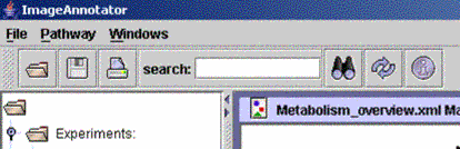
| After starting the MapMan software you will find data
files in the Experiments folder, pathway image files in the
Pathways(overview of available predefined pathways)folder and mapping files in the Mappings folder of the
selection directory on the left. You can view the included datasets in context of different metabolic pathways |
||
| (i)Double click an image file from the folder "Pathways", | |
 |
e.g. "Metabolism_overview" or "Glycolysis". Choose a mapping file from the pop-up box and click "OK". Choose "AFFY2005" in combination with "Metabolism_overview" with all maps showing biological processes (This is most often right). Hint: Images need different mapping files (table 1). Response_images need an Response_mapping file. (In fact, if you don’t care about the statistics you can combine both files). |
| (ii) The diagram is depicted in the right MapMan window. |
 |
| (iii) A simple click activates experiment files from the folder | |
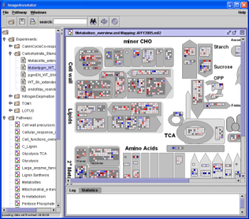 |
"Experiment:DiurnalCycle
(or other) one by one. All data files from one experiment can now be
viewed in sequence. Each file is called up after loaded the first time
by mouse click in a fraction of a second. Each gene is symbolised by a box, the gene expression level is colour-encoded (red = down-, blue = upregulation). |
|
A simple mouse-over action on an individual box will call up the gene annotation beneath your mouse,
while a click will copy the information to the text window below pathway. Right clicking on an individual box brings up further options, such as opening a webbrowser (link out) with additional information about the particular spot from the GABI website (http://www.gabipd.org) which will also get you to further information ressources. You can get unigene information, and information how good a spot reflects a given transcripts. |
|
| Number | Filename | Description/Keywords | Visualization | Data | Standard/ Response |
| 1 | photosynthesis | Light reaction, Calvin cycle, photorespiration | P | T | S |
| 2 | cell functions overview | cellular functions | H | T | S |
| 3 | Cell Wall precursors | NDP sugar pathways (used for the cell wall) | P | T | S |
| 4 | Cellular reponse overview | stresses, redox, development, cell cycle and division | P | T | S |
| 5 | Glycolysis | glycolysis | P | T | S |
| 6 | Large enzyme families | Large enzyme families like oxidases, GDSL lipases, etc | P | T | S |
| 7 | Lignin | Monolignol pathway starting from Phenylalanine | P | T | S |
| 8 | metabolism overview | overview of metabolic reactions | P | T | S |
| 9 | mitochondrial e-transport | mitochondriol overview including transporters | P | T | S |
| 10 | N-metabolism | Nitrogen metabolism | P | T | S |
| 11 | RNA-Protein Synthesis | Protein Synthesis, targeting and degradation as well as RNA processing |
P/H | T | S |
| 12 | Sucrose Starch | Sucrose and Starch Degradation and Synthesis | P | T | S |
| 13 | Transcription Regulation | Potential Transcription factors and regulators of transcription | P | T | S |
| 14 | Transport Overview | different transporters | P | T | S |
| 15 | Proteasome | Ubiquitin dependent protein degradation pathway | P | T | S |
| 16 | Regulation overview | TFs, Protein modification and degradation, hormone regulation, receptor kinases, G proteins, MAPKs etc. |
P | T | S |
| 17 | TCA | TCA Cycle including mitochondrial genes | P | T | S |
| 18 | Glycolysis-TCA | Combination of Glycolysis, TCA, and mitochondrial genes | P | T | S |
| 19 | Secondary metabolism | Secondary metabolism like flavenols, chalcones, lignins, etc | P | T | S |
| 20 | Pentose phosphate | Pentose phosphate pathway, Warburg way, Shunt | P | T | S |
| 21 | Metabolites | most metabolites that can be measured, for a conversion of your metabolite name to the canonical MM one see: http://csbdb.mpimp-golm.mpg.de/csbdb/gmd/tools/gmd_conv.html |
P | M | S |
| 22 | C_TCA | only the TCA cycle including some metabolites | P | T/M | S |
| 23 | Sulfate assimilation | Sulfate assimilation | P | T | S |
| 24 | C_Lignin | Monolignol pathways (slightly different layout as ligin with transcript only) | P | T/M | S |
| 25 | Response_nutrients | Response to starvation and readdition of nutrients: phosphate, nitrate, sulphate, carbon |
P | T | R |
| 26 | Response_stress | Response to abiotic stresses from Atgenexpress (roots) | P | T | R |
| Visualization types: P(oints) H(istogram) | |||||
| Data types: T(ranscripts) M(etabolites) P(roteinas) | |||||
| Table 1:Available image, mapping and experiment
files. Regard: Some of the mapping files included in this package might be encrypted. To receive the original files, please contact: Mark Stitt (stitt@mpimp-golm.mpg.de) |
|||||
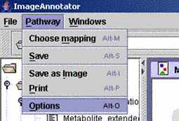
| 1.2 Display options | index | |||
| In default mode, each individual gene (protein,
metabolite) is symbolised by a small square box in which the expression
(concentration) level is colour-encoded. In case of gene expression experiments, up-regulated genes are shown in blue, while down-regulated genes are stained in red. [Colour coding will be extended with planned additions] The display options can be changed: |
||||
| (i) Select "Options" from the "Pathway" menu. | ||||
 |
||||
| (ii) Scaling: Change the colour intensity of your data points. Scale down the value for more, scale up the value for less colour intensity. The default value is 3.0. Datasize: Minimize or enlarge the box size. Middle size (M) is default value. Background Colour: Change the colour of the image background. |
 |
|||
|
Visualization Type: Change mode, default means use visualizations as specified for each data area, other modes override the modes specified for each data area Marked Visualization Type: Change visualization for marked elements. You will only notice changes in visualization for marked elements which have been marked via the search function! |
||||
| 1.3 Print | index | |
| Print your image-data-file: Select "Print" from the "Pathway" menu. |
||
| 1.4 Save | index | |
| You can save the result of an experiment depicted on a
pathway as an image-data-file: Select "Save as Image" from the "Pathway" menu. It is possible to save the image as .jpg or .png file. After selecting a file-type write the filename and add the correct ending of the file name (.jpg or .png). |
||
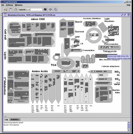
| 1.5 Search Functions | index | |
| The search function allows you searches in the description for all genes/metabolites/proteins which are present on a selected pathway. | ||
| Type in the your search description in the search field. Press the binocular button right beside the search field to start. In the "Log" tab ( bottom pane )the number of found matches is displayed. Additionally, all spots which were matched by the search are displayed according to the selected display options from the menu: "Pathway->Options->MarkedVisualiationType". (The experienced user can make use of regular expression a.k.a. REGEX syntax) Press the recycle button to reset the marking on the pathway diagram |
||
 |
||
|
Results of all matches are visually highlighted in each individual box. The displayed visualization can be altered under the options menu, selecting other options under "e;MarkedVisualizationType"e;. The default display is "e;3D rectangles"e; In the example shown, the option "e;greying"e; was chosen, the greys out all items that do not match with the descriptor search of interest. Other available search options are "e;Inner Rectangles"e;, "e;Triangles"e; and "e;3D Rectangles"e;. The Highlighting option can be modified under Pathways->Options->MarkedVisualizationType. See paragraph 1.2 |
||
 |
||
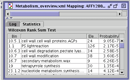
| 1.6 Statistics (Wilcoxon Rank SumTest) | index | |
|
The statistics performed in MapMan is based on the Wilcoxon Rank Sum
Test to predict BINs that exhibit a different behaviour in
terms of expression profile compared to all the other remaining
BINs. The test is done automatically every time a new experiment is loaded. For each BIN the results are displayed (BIN, Elements, Probability) in the Statistics panel beside the Log panel at the bottom pane below the pathway diagram. |
||
 |
||
The test is done automatically every time a new experiment is loaded. For each Bin displayed the results (Bin, Elements, Probability) of the test is shown in the Statistics panel beside the Log panel at the bottom part of the pathway. |
||
| 2 View your own Arabidopsis 22K Affymetrix data | index | |
|
Users of MapMan can visualize their own Arabidopsis 22K Affymetrix
microarray experiments using the mapping and pathway image files
included in the MapMan package. New files with experimental data have to be in a specific format (2.1) and are loaded into MapMan in two steps. The first step is to create a new experiment subdirectory folder (2.2) and the second step is to upload data files into this folder (2.3). You are able to create as many experiment folders as you like and reference data files belonging to your experiment. |
||
| 2.1 Data format | index | |||||||||||||||||||||||||||||||||||
| The data format MapMan expects is either an EXCEL or tab-delimited text file. Files might have the following structure: Values should typically be in the range of -10 to 10, but values may be higher or lower). | ||||||||||||||||||||||||||||||||||||
| Single assay file format: | Multiple assay file format: | |||||||||||||||||||||||||||||||||||
|
|
|||||||||||||||||||||||||||||||||||
| ¹Values of 'X' mean absent, which will be displayed as empty squares. | ||||||||||||||||||||||||||||||||||||
|
The "IDENTIFIER" - column refers to the unique EST or
oligo sequence identifier. For example Affymetrix Identifiers
represented on your filter/array. The "VALUE" - column indicates for each identifier the measured expression value. A negative/positive value represents downward/upward regulation. We recommend using logarithms of measured expression ratios between two treatment conditions in an experiment (e.g. log2 expression values representing fold change). MapMan expects numeric information in the "VALUE" column to be within the range -10 to 10, but values may be higher or lower. Missing or absent values are marked by a capital "X". Alternatively MapMan can load files containing multiple assays at once. MapMan expects the Probe identifier in the first columns, all following columns contain the individual experiment values. The tables can contain a header with the name of the experiment, but this is not necessary. |
||||||||||||||||||||||||||||||||||||
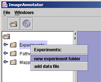
| 2.2 Create an experiment (folder) | index | |
|
Experimental data can be organized in folders and data files can than be added to those folders. Alternatively folders from the file system can be selected and the containig data files will be added automatically. |
||
|
(i) Right click on any experiment folder in the folder structure on the left pane, and select "new sub folder" to generate a new experiment folder in MapMan |
 |
|
|
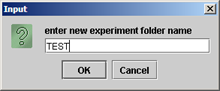
(ii) An option box appears: Select"by name" to add files individually. (Advanced users can optionally reference directories by selecting existing folders to load all data files within a given directory) |
 |
|
|
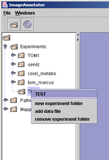
(iii) The new experiment folder will show up in the folder structure: |
 |
|
| 2.3 Add data files to your new folder | index | |
|
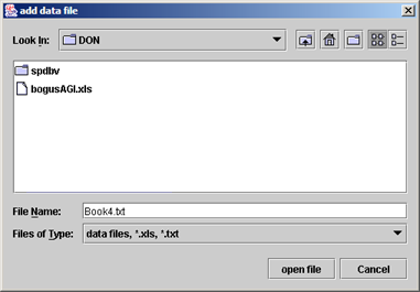
(i) Right click the mouse button on the newly created experiment folder and select "add data file" from the menu. |
 |
|
|
(ii) Choose your data files one by one. (Tab delimited text files are much faster to load than excel files!) You can export your data from excel as tab delimited text files. |
 |
|
|
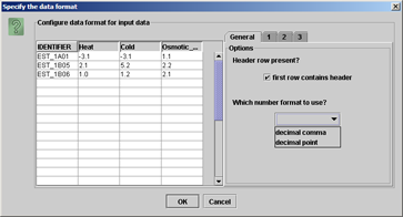
(iii) A dialog opens giving the option to configure your datafile. You have the option to deselect data columns you are not going to use which will speed up loading of the data and prevent errors from unreadable data. |
||
|
Usually MapMan does recognize the format of your data automatically. (Check if the number format matches (decimal point or comma)) Moreover, you can force MapMan to take a header row or not to take a header, by checking or unchecking the check box "first row contains header" respectively. |
 |
|
|
(iv) All configured data files are now listed within your experiment folder. | 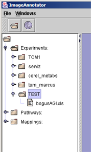 |
|
| 2.4 Visualise your data | index | |
| Once you have imported your data file into MapMan it is possible to display these data sets onto an image (diagram). Please follow the instructions as outlined in paragraph 1. | ||
| 3 Use MapMan to visualise any gene expression, metabolite or other data | index | |
| In general MapMan can be used to display any data onto
user-defined images. Data can be gene expression data, metabolite or
protein concentrations, enzyme activities etc. Image files (.png, .bmp ?) can be metabolic pathways, cellular processes, regulatory networks etc. Prior MapMan usage two steps are necessary: (i) creation of a mapping file (3.1), (ii) annotation of new image files (3.2). |
||
| 3.1 Creation of a custom mapping file | index | ||||||||||||||||||||||||||||||||||||||||||||||||||||||||
| The mapping file structures your genes, metabolites,
enzymes etc. in discrete classes in a hierarchical way. The mapping
file has to be in "MS-EXCEL", tab-delimited ".txt" or ".xml"
format. Define the five firest columns as "BINCODE", "NAME", "IDENTIFIER" , "DESCRIPTION", "TYPE". The "BINCODE" column contains the identifier for all your main classes (1, 2, 3, 4 ....), subclasses (1.1, 1.2, ...., 2.1, 2.2....), subsubclasses (1.1.1, 1.1.2....1.2.1, 1.2.2.....) and so on. Important is the dot between classes and their subclasses. The BINCODE is used to annotate the image files (3.2). The "NAME" column includes the names for each class (e.g. Photosynthesis) and subclass (e.g. Photosynthesis.lightreaction). Again a dot separates classes and subclasses. The "IDENTIFIER" column lists the identifier of a gene, metabolite, enzyme etc.. These identifiers have to match the identifier in your data file. The "DESCRIPTION" column contains a user-defined description of the gene, metabolite, enzyme etc. There is no space limitation. The "TYPE" column specifies if the item is a transcript (T), metabolite (M), enzyme (E), protein (P) Hint: Currently you can leave out the Type column for backward compatibility reasons |
|||||||||||||||||||||||||||||||||||||||||||||||||||||||||
|
|||||||||||||||||||||||||||||||||||||||||||||||||||||||||
| Table 2: Example for a .xls mapping file. | |||||||||||||||||||||||||||||||||||||||||||||||||||||||||
|
Regard : Some of the mapping
files, included in the package might be encrypted. Please contact Mark Stitt (stitt@mpimp-golm.mpg.de)to get one of the original mapping files. |
|||||||||||||||||||||||||||||||||||||||||||||||||||||||||
| 3.1.1 Add mappings to the "Mappings" folder | ||
| Once a new mapping file is created it can be loaded into MapMan: | ||
|
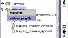
(i) Right mouse click on "Mappings" and then "Add mapping file". Select your newly created .txt, .xls or .xml file from the folder source. |
 |
|
| (ii) A box appears: | ||
| Select | "from file" to add files individually | 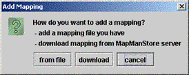 |
| or | "download" to add mapping files from the MapManStore server which has updated mappings. | |
| (iii) Select the appropriate mapping file | ||
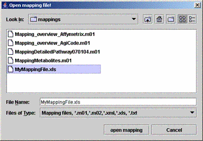 |
||
| (iv) The mapping name is shown in the "Mappings" tree structure without the file extensions .txt or .xls. | 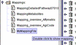 |
|
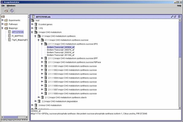
| (v) By double click the mapping file is
displayed and it is possible to browse through this file. A mouse click on the (sub)classes or identifier shows up the information as outlined in the "DESCRIPTION" field of your mapping file as well as the "TYPE" of your spot: |
||
 |
||
| 3.2 Create your own pathway (Annotation of an image file) | index | |
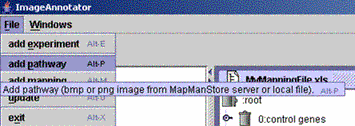
| (i) Select "Add pathway" from the "File" menu and select an image file from your directory. The new file will appear in the "Pathways" folder in the left pane. | ||
 |
||
| (ii) To annotate the new image click the right mouse button on the image where you want to place your annotation and select "add" from the "Annotation" menu. | 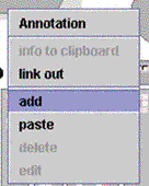 |
|
| (iii) A dialog box is opened in which the user is asked to type in the numerical identifier of the BINS/subBINS for which data should be deposited, concordant to your mapping file.The "Block Format" can be set: type in xa or ya (a=1...n). This format assigns the arrangement of the boxes (if default or points is chosen as "Visualization Type") | ||
E.g. Block Format x20 Block Format y16  |
 |
|
| Visualization Type histogram (3.3) Choose "histogram" as "Visualization type" to view data in a histogram frequency chart. |  |
|
| (iv) You can specify what kind of data you want to show. Currently ImageAnnotator supports four different kinds of data points that can be nested. However, you have to have a mapping file that supports these different data types. | 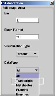 |
|
| Annotated areas are marked by a dot and can be moved to exactly adjust the position via mouse dragging (holding down the left mouse key on a annotation dot and moving the mouse). It can also be achieved by clicking on the annotation dot and afterwards holding down the alt key and using the arrow keys for positioning. Add as many annotations points to the image as you want. | ||
| All annotation points can be changed or deleted: (i) To change the annotation text or to switch to the histogram frequency chart, click the right mouse button on the point you want to change and select "Edit" from the menu. Type in your changes. (ii) To delete an annotation just click on the point with the right mouse button and select "Delete". |
||
| 3.3 Histogram frequency chart | index | |
| The genes (enzymes, proteins) in a selected group can be treated as a population , and their collective response displayed as a frequency histogram. Genes (enzymes, proteins) that change by less than a filter value (e.g., <0.33 and >-0.33 on a log scale 2) are grouped into the central white bar, genes that increase are displayed as a series of blue bars at right hand side (corresponding on this scale to changes between 0.33-0.99, 0.99-1.66, 1.66-2.33, 2.33-3.00 and >3.0 respectively), and genes that decrease are shown by a similar set of red bars on the left hand side. | ||
| 4 Structure of Mapman | index | |
| MapMan relies on SCAVENGER modules to build mapping files. These SCAVENGER modules group metabolites, transcripts etc. data into the BINS. The SCAVENGER modules are completely independent of the ImageAnnotator module and vice versa. The ImageAnnotator module uses mapping files from the SCAVENGER modules or user-built mapping files as its data source. It then paints out the experimental data onto maps (images with accompanying XML files) according to the hierarchical structure of the mapping files. | ||
 |
||
| 6 Contact information | index | |
Axel Nagel (application design, software development)  GABI Primary Database Max Planck Institute of Molecular Plant Physiology Am Muehlenberg 1 D-14476 Golm |
||
| Bjoern Usadel, usadel@mpimp-golm.mpg.de (annotation computing, pathways) Max Planck Institute of Molecular Plant Physiology Am Muehlenberg 1 D-14476 Golm |
||