|
|
 |
SATlotyper FAQ |
Haplotype inference from unphased SNP data in heterozygous polyploids based on SAT |
|
Contents:
|
|
|
|
|
How is SATlotyper started?
|
|
First of all, SATlotyper is written in Java which means that Java Runtime Environment 1.5.0 or higher must be installed on your computer.
You can test if Java is installed on your computer by typing "java" into a command prompt (command line):
Windows
1. click "start" and then "run"
2. insert "cmd" into the upcoming box and press enter
3. insert "java" into the upcoming black box and press enter
4. insert "java -version" and press enter
Linux/Mac
1. start a terminal, insert "java" and press enter
2. insert "java -version" and press enter
Independently of the operating system, if no error message occurs, a Java Runtime Environment is installed.
If no Java Runtime Environment is installed, download it from Sun and install it or ask your administrator to do it for you.
If all these requirements are fulfilled you can start SATlotyper:
Windows
1. unzip the SATlotyper_v0.1.5.zip file
2. enter the SATlotyper_v0.1.5 directory and double-click on SATlotyperGUI.jar
Linux/Mac
1. unzip the SATlotyper_v0.1.5.zip file
2. enter the SATlotyper_v0.1.5 directory
3. type "java -jar SATlotyperGUI.jar" and press enter
Independently of the operating system, the following window comes up:
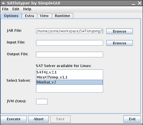
The shown GUI above is only an interface to SATlotyper, the actual program is the SATlotyper.jar file.
After entering the SATlotyper_v0.1.5 directory, you can test the program on command line:
type "java -jar SATlotyper.jar" and press enter.
|
|
Go To Top
|
|
|
|
|
|
How is the GUI organized?
|
|
|
The GUI consists of four panels: Options, Extra, View and Runtime.
The Options panel manages the necessary information for SATlotyper, for instance in- and output files or the SAT solver.
On the Extra panel the user can select and change parameters which SATlotyper provides.
The View panel provides a convenient way to browse the data of the input file as well as the resulting data.
Since the GUI is only an interface to SATlotyper, the Runtime panel shows the command line output of SATlotyper.
|
|
Go To Top
|
|
|
|
|
|
Which file formats are supported?
|
|
The current version of SATlotyper can read so called CSV files.
A CSV file is a convenient way for representing a table.
A row in the file represents a row of the table.
The columns of a row are separated by a "," or an other character (e.g. ";" or a tab).
The content of a cell may be enclosed by """ or "'".
An example file can be found here, where columns are separated by tabs.
If your data is saved as XLS file, you can easily transform it to a CSV file by selecting the corresponding file ending when you save your data with Excel/OpenOffice again.
Note that a CSV file can only handle one sheet.
If your Excel/OpenOffice file consists of more than one sheet, you must save each sheet as a new CSV file.
If you convert your data to a CSV file and SATlotyper loads the data, very often an file format error is reported.
This error occurs because the original Excel/OpenOffice files often contain characters like " ".
Not visible characters are inserted to the data when the file is intensively edited by hand.
Such characters become visible if you save your data as CSV file where the content of the cells is enclosed by """.
Note that the result of a computation is saved as XML file which you can also use as input.
Furthermore, the data stored in the XML file can be browsed on the View panel.
|
|
Go To Top
|
|
|
|
|
|
What is the Options panel good for?
|
|
|
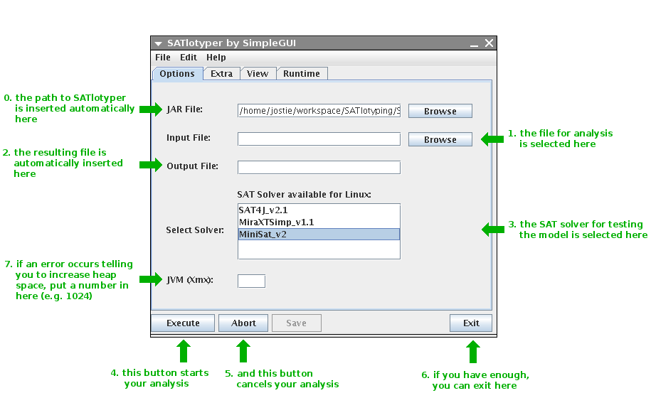
The Options panel is the most important one.
Here you define the input file, the SAT solver you want to use as well as how much memory SATlotyper is allowed to use:
|
|
|

0. Here, you define where the SATlotyper program is located.
This field is filled automatically and should not be changed.
1. When the Browse button is pressed, a new dialog box is opened with which you can select the input CSV file.
2. The resulting XML file is inserted into this field automatically.
You will find the file at the corresponding directory on your file system.
3. Here, you can select the SAT solver you want to use.
There are several different SAT solvers available corresponding to your operating system.
4. If you press this button, the program will start with the computation.
5. You can always abort the computation by pressing the Abort button.
6. If you want to exit, press the Exit button.
7. By default, the Java Runtime Environment provides a predefined amount of memory to all Java programs.
If the needed memory for encoding an input file exceeds this predefined amount of memory, an error is reported by SATlotyper.
Insert a large number into this field (e.g. 1024).
Clearly, your computer must provide the inserted amount of memory in MB!
|
|
Go To Top
|
|
|
What is the Extra panel good for?
|
|
The Extra panel allows the user to change different parameters:
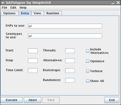
SNPs to use: Here you can explicitly select a subset of SNPs.
For instance, if your dataset contains 20 SNPs and you want to analyze the first 10 SNPs, enter 1,2,3,4,5,6,7,8,9,10 into the corresponding field.
Genotypes to use: Here you can explicitly select a subset of genotypes, analogous to "SNPs to use".
If your dataset contains many genotypes it may be better to edit your dataset with Excel/OpenOffice and save it as a new smaller CSV file.
Start and Stop: If you know that the number of haplotypes is greater (or equal) x and a less (or equal) y, you can enter this information into the corresponding fields.
Timelimit: If you want to abort the computation after some predefined amount of time, you enter this value (in seconds) here.
Threads: If you use a multithreaded SAT solver (e.g. MiraXT) you can define the number of threads in this field.
Alternatives: Forces the program to compute the given number of alternative most parsimonious inferences.
Bootstraps: Forces the program to compute the given number of bootstrap samples.
This makes only sense in combination with computing alternatives.
Randomize: If the SAT solver provides the possibility to compute inferences drawn randomly from the set of valid solutions (e.g. MiniSat) you can enter a value between 0 and 1 here.
Include Alternatives: If this checkbox is activated, the alternative inferences are treated as bootstrap samples.
Optimize: If activated, the genotype inferences of each computed solution is optimized in respect to the bootstrapping scores.
This makes only sense in combination with computing alterantives and bootstrap samples.
Verbose: If activated and the used SAT solver has a command line output, this output is shown on the Runtime panel.
Show All: If activated, the inference of genotypes is reported additionally to the inference of haplotypes on the Runtime panel.
|
|
Go To Top
|
|
|
What is the View panel good for?
|
|
The View panel provides a convenient way to browse the data of the input file as well as the resulting data:
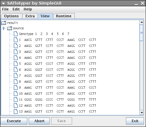
The browsing can easily be done by expanding and collapsing the shown tree.
|
|
Go To Top
|
|
|
What is the Runtime panel good for?
|
|
Since the GUI is only an interface to SATlotyper, the Runtime panel shows the command line output of SATlotyper:
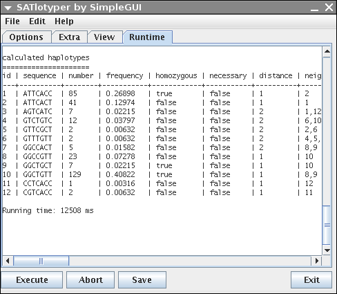
You can save the output by clicking on the Save button.
If an inference was calculated, a short statistic lists the resulting hapltoypes in a table.
The table contains 8 columns (id, sequence, number, frequency, homozygous, necessary, distance, neighbours).
The last three columns need some explanation.
The necessary column is deprecated and contains no usefull information for the user.
The distance column represents the distance of the corresponding haplotype to its nearest neighbouring haplotype.
The distance is defined as the minimal necessary number of mutations for deriving haplotype x from haplotype y.
The last column lists the nearest neighbours (given as id) to the corresponding haplotype.
|
|
Go To Top
|
|
|
What about missing values?
|
|
If your data also contains SNP sites for which no allele information is available, mark the position with Ns in the CSV file.
For instance, SNP 1 of a tetraploid and biallelic dataset contains the alleles A and G.
Suppose further that the allele composition of genotype 20 is not known at position 1.
Such data can be easily completed by using allele composition NNNN for genotype 20 at position 1.
The corresponding SNP or genotype needs not to be removed from the dataset.
An example can be found here.
Furthermore, if the allele dosage is not known for a given SNP and genotype, mark the remaining alleles with Ns.
For instance, SNP x of a tetraploid and biallelic dataset contains the alleles G and T.
Suppose further that the allele dosage of genotype y is not known at position x but it is known that allele G and T are present.
Such data can be easily completed by using allele composition GTNN for genotype y at position x.
The corresponding SNP or genotype needs not to be removed from the dataset.
An example for a hexaploid species can be found here.
|
|
Go To Top
|
|
|
What if the computation does not stop?
|
|
|
The inference of unphased genotypes into haplotypes is very hard to compute.
Given two, on the first sight similar datasets, the first inference might be reported in seconds whereas the second inference can not be computed at all.
For the second case, stop the computation and reduce the number of SNP sites or genotypes.
|
|
Go To Top
|
|
|
|
|
|


